Making Fractals in GeoGebra

Here you can find some hints for making fractals using GeoGebra software. This is how I made the images on my fractal art page.

Many fractals are formed by performing some simple action over and over again, in a sequence of recursive steps. At each step the input is some simple shape – a polygonal curve, say – and the output is some modification of that shape.

The Cantor Set

The most simple example is the Cantor set. Beginning with a line segment, we remove the middle third, resulting in two segments. We repeat this same action on each of these segments, resulting in four. At the next step we have eight, and then sixteen. This continues ad infinitum (or as long as the limitations of our computer will allow).

Click here for an animation.

Let's construct this on GeoGebra. Begin with an arbitrary line segment a. The Point function allows us to select any point along the length of a; Point[a,0] is the initial endpoint, and Point[a,1] is the terminal endpoint. To remove the middle third of a, we replace it with the two segments

Segment[Point[a,0],Point[a,1/3]]

Segment[Point[a,2/3],Point[a,1]]

Note that this amounts to two commands. Think about it. If we go about our process like this, at each step the number of commands will have to double, and the amount of work we're doing will increase at an exponential rate. That's not good! We need a way of performing each step with a single command. But that's easy: use a list. Our command will be

{Segment[Point[a,0],Point[a,1/3]],Segment[Point[a,2/3],Point[a,1]]}

which results in the pair of line segments: {*,*}. Now, at each stage we want the output to have the same form as the input, so we should begin, not with a single line segment, but with a list containing a single line segment: {*}. Then at each stage the input and the output will be lists of segments.

So let's start over: list1 will be the list {a}, and list2 will be

{
     Segment[
          Point[a,0],
          Point[a,1/3]
     ],
     Segment[
          Point[a,2/3],
          Point[a,1]
     ]
}

Then list3 will be created by performing the same action on each of these segments. They aren't named, but we can access them through the Element function. Element[list2,1] is the first segment, and Element[list2,2] is the second. So list3 is

{
     Segment[
          Point[Element[list2,1],0],
          Point[Element[list2,1],1/3]
     ],
     Segment[
          Point[Element[list2,1],2/3],
          Point[Element[list2,1],1]
     ],
     Segment[
          Point[Element[list2,2],0],
          Point[Element[list2,2],1/3]
     ],
     Segment[
          Point[Element[list2,2],2/3],
          Point[Element[list2,2],1]
     ]
}

This accomplishes what we desire, but is still unsatisfactory. The amount of typing is still going to double at each stage if we have to enter the segments by hand. We need a way of making the computer read through them on its own. This can be done with the Sequence command. The entry

Sequence[F(k),k,1,n]

returns the list

{F(1),F(2),…,F(n)}

where F is some function accepting an integer as an argument. In our case, the n should be the number of elements in list2, or Length[list2]. The function should return the pair of segments resulting from removing the middle third from Element[list2,k] for each k, or

{
     Segment[
          Point[Element[list2,k],0],
          Point[Element[list2,k],1/3]
     ],
     Segment[
          Point[Element[list2,k],2/3],
          Point[Element[list2,k],1]
     ]
}

If we use this as our F(k), the output will be of the form {{*,*},{*,*}}. However, we want a list of segments, not a list of pairs of segments. So after running through the sequence we'll apply the Join command, resulting in {*,*,*,*}. Thus:

Join[
     Sequence[
          {
               Segment[
                    Point[Element[list2,k],0],
                    Point[Element[list2,k],1/3]
               ],
               Segment[
                    Point[Element[list2,k],2/3],
                    Point[Element[list2,k],1]
               ]
          },
          k,
          1,
          Length[list2]
     ]
]

So our input should read

list3=Join[Sequence[{Segment[Point[Element[list2,k],0],
Point[Element[list2,k],1/3]],Segment[Point[Element[list2,k],2/3],
Point[Element[list2,k],1]]},k,1,Length[list2]]]

To be consistent, we could start by defining list2 this way:

list2=Join[Sequence[{Segment[Point[Element[list1,k],0],
Point[Element[list1,k],1/3]],Segment[Point[Element[list1,k],2/3],
Point[Element[list1,k],1]]},k,1,Length[list1]]]

Then list3 would be defined as above, and next we would have

list4=Join[Sequence[{Segment[Point[Element[list3,k],0],
Point[Element[list3,k],1/3]],Segment[Point[Element[list3,k],2/3],
Point[Element[list3,k],1]]},k,1,Length[list3]]]

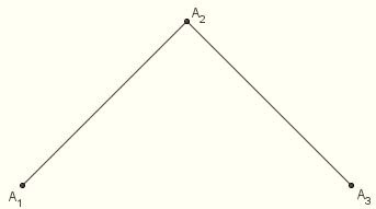
and so on, creating list5, list6, etc. Hide all but the last stage to see a good picture of the Cantor set. (There's not much to see. Although the Cantor set is uncountable, it has measure zero.)

As a fun variation, begin with two concentric circles c = Circle[A,B] and d = Circle[A,C]. Place a point D on c. Let E be the intersection betwee Ray[A,D] and d. Perform the Cantor set construction using a = Segment[D,E]. Hide all but the last list. Set the list to "Trace On," and set D to "Animation On." Does the shape that's traced remind you of anything? (It's been proposed that the Cantor set models the rings of Saturn.)

The Harter-Heighway Dragon Sweep

The dragon sweep is illustrated on my fractal art page; please click here for a description.

Beginning with an "elbow" (a pair of line segments of equal length, sharing a common endpoint, with an angle of 90° between them), we replace the first segment with an "elbow" of the opposite orientation, and the second with an "elbow" of the same orientation, resulting in four segments. Then we repeat the process for these four segments, alternating between the two types of elbows. And so on, ad infinitum. This results in the sweep.

Click here for an animation.

Let's construct the sweep on GeoGebra. We start out with three points A₁, A₂, and A₃ which form a left-handed "elbow" as shown.

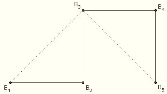
We connect them with a polygonal curve (a "polyline"):

step1 = PolyLine[A1,A2,A3]

At each step we begin with such a polyline. We go through the polyline one segment at a time and replace them all with elbows: first a right-handed elbow, then a left-handed elbow, alternating like this until we reach the last segment.

Consider step1. The first vertex of step2 should be A₁; let's rename it B₁.

B₁ = A₁

The next vertex is the corner of the right-handed elbow, i.e., the corner of the square with diagonal A₁A₂. The Pythagorean Theorem tells us that its distance from A₁ is 1/sqrt(2) ⋅ A₁A₂. So to obtain it we rotate A₂ clockwise about A₂ through an angle of 45° and dilate by a factor of 1/sqrt(2). First we rotate, then we dilate. We'll call this point B₂. So

B₂ = Dilate[Rotate[A₂,315°,A₁],1/sqrt(2),A₁]

(The Rotate function only accepts positive angle values, so here we rotated counter-clockwise through 315° rather than clockwise through 45°.) The third point is A₂:

B₃ = A₂

The fourth point (the corner of the second elbow) we obtain by rating A₃ counter-clockwise about A₂ through an angle of 45° and dilating by a factor of 1/sqrt(2):

B₄ = Dilate[Rotate[A₃,45°,A₂],1/sqrt(2),A₂]

And the last point is A₃:

B₅ = A₃

So our next iteration is:

step2 = PolyLine[B₁,B₂,B₃,B₄,B₅]

Let's review:

B₁ = A₁
B₂ = Dilate[Rotate[A₂,315°,A₁],1/sqrt(2),A₁]
B₃ = A₂
B₄ = Dilate[Rotate[A₃,45°,A₂],1/sqrt(2),A₂]
B₅ = A₃
step2 = PolyLine[B₁,B₂,B₃,B₄,B₅]

The third polyline is formed in much the same way. Replace B₁B₂ with a right elbow, B₂B₃ with a left elbow, B₃B₄ with a right elbow, B₄B₅ with a left elbow, as before. So:

C₁ = B₁
C₂ = Dilate[Rotate[B₂,315°,B₁],1/sqrt(2),B₁]
C₃ = B₂
C₄ = Dilate[Rotate[B₃,45°,B₂],1/sqrt(2),B₂]
C₅ = B₃
C₆ = Dilate[Rotate[B₄,315°,B₃],1/sqrt(2),B₃]
C₇ = B₄
C₈ = Dilate[Rotate[B₅,45°,B₄],1/sqrt(2),B₄]
C₉ = B₅
step3 = PolyLine[C₁,C₂,C₃,C₄,C₅,C₆,C₇,C₈,C₉]

Hopefully now we can start to see a pattern emerging. The goal is to come up with a single command that will take step(n) as its input and yield step(n+1) as its output.

Observe that lines 1 through 4 in the formation of step2 are repeated in lines 1 through 4 and lines 5 through 8 of step3. We would imagine that the same sequence is repeated four times in the formation of step4 (since step3 has four elbows). The sequence looks like this:

D_4k-3 = C_2k-1
D_4k-2 = Dilate[Rotate[C_2k,315°,C_2k-1],1/sqrt(2),C_2k-1]
D_4k-1 = C_2k
D_4k = Dilate[Rotate[C_2k+1,45°,C_2k],1/sqrt(2),C_2k]

This gets repeated four times (for k = 1, 2, 3, 4). Then the last vertex is defined as D₁₇ = C₉. Now, we want our input to be step3, not C₁ through C₉. We can avoid referring to the points by name if we use the Vertex command. For instance, the command

Vertex[step3,n]

returns the n^th vertex of the polyline step3, which happens to be C_n. So we can replace our sequence with

Vertex[step3,2k-1]
Dilate[
     Rotate[Vertex[step3,2k],315°,Vertex[step3,2k-1]],
     1/sqrt(2),
     Vertex[step3,2k-1]
]
Vertex[step3,2k]
Dilate[
     Rotate[Vertex[step3,2k+1],45°,Vertex[step3,2k]],
     1/sqrt(2),
     Vertex[step3,2k]
]

We want to repeat this for k = 1, 2, 3, 4. However, the output needs to be a single object, not four objects. So, instead of outputting four points, we output a single sequence of four points:

{
     Vertex[step3,2k-1],
     Dilate[
          Rotate[Vertex[step3,2k],315°,Vertex[step3,2k-1]],
          1/sqrt(2),
          Vertex[step3,2k-1]
     ],
     Vertex[step3,2k],
     Dilate[
          Rotate[Vertex[step3,2k+1],45°,Vertex[step3,2k]],
          1/sqrt(2),
          Vertex[step3,2k]
     ]
}

We do this for k = 1, 2, 3, 4, which is accomplished as follows:

Sequence[{*,*,*,*},k,1,4]

We want our script to work for any step, not just step3. In general, the number of vertices in the polyline step(n) is p = 2n + 1, while the number of times we repeat this sequence in step(n+1) is q = 2n – 1. So

q = (p – 1)/2

Now, m itself is the number of vertices in step(n), which we can get at by using the Vertex function. {Vertex[*]} returns the set of vertices as an ordered list, so

p = Length[{Vertex[step3]}]

q = (Length[{Vertex[step3]}]-1)/2

and our sequence looks like

Sequence[{*,*,*,*},k,1,(Length[{Vertex[step3]}]-1)/2]

This generates a sequence of sequences of points. In the case of step4, it looks like this:

{{D₁,D₂,D₃,D₄},{D₅,D₆,D₇,D₈},{D₉,D₁₀,D₁₁,D₁₂},{D₁₃,D₁₄,D₁₅,D₁₆}}

The function PolyLine takes a sequence of points as its argument, not a sequence of sequences. We could use the Join function to combine these into a single sequence:

Join[{{D₁,D₂,D₃,D₄},{D₅,D₆,D₇,D₈},{D₉,D₁₀,D₁₁,D₁₂},{D₁₃,D₁₄,D₁₅,D₁₆}}]

which would result in

{D₁,D₂,D₃,D₄,D₅,D₆,D₇,D₈,D₉,D₁₀,D₁₁,D₁₂,D₁₃,D₁₄,D₁₅,D₁₆}

But we still need to add D₁₇. We can accomplish this by joining the list {D₁₇}:

Join[{{D₁,D₂,D₃,D₄,D₅,D₆,D₇,D₈,D₉,D₁₀,D₁₁,D₁₂,D₁₃,D₁₄,D₁₅,D₁₆},{D₁₇}}]

Now, D₁₇ is simply the last vertex of step3, so it can be written as

Vertex[step3, Length[{Vertex[step3]}]]

We're ready to form our polyline. Thus:

PolyLine[
     Join[
          {
               Join[
                    Sequence[
                         {
                              Vertex[step3,2k-1],
                              Dilate[
                                   Rotate[Vertex[step3, 2k], 315°,Vertex[step3, 2k - 1]],
                                   1/sqrt(2),
                                   Vertex[step3,2k-1]
                              ],
                              Vertex[step3, 2k],
                              Dilate[
                                   Rotate[Vertex[step3, 2k+1],45°,Vertex[step3, 2k]],
                                   1/sqrt(2),
                                   Vertex[step3,2k]
                               ]
                          },
                         k,
                         1,
                         (Length[{Vertex[step3]}] - 1)/2
                    ]
               ],
               {
                    Vertex[step3, Length[{Vertex[step3]}]]
               }
          }
     ]
]

All together, our input is

step4=PolyLine[Join[{Join[Sequence[{Vertex[step3,2k-1],
Dilate[Rotate[Vertex[step3,2k],315°,Vertex[step3,2k-1]],
1/sqrt(2),Vertex[step3,2k-1]],Vertex[step3,2k],
Dilate[Rotate[Vertex[step3,2k+1], 45°,Vertex[step3,2k]],
1/sqrt(2),Vertex[step3,2k]]},k,1,(Length[{Vertex[step3]}]-1)/2]],
{Vertex[step3,Length[{Vertex[step3]}]]}}]]

To perform the next step, simply replace step3 with step4. And so on.